The first version of this renderer is a CPU ray caster: a Scene::TraceImage that walks every pixel, generates a primary ray, asks the scene for the closest hit, and writes whatever that hit reports as color. No light, no bounces, no global illumination — just the closest-hit query. The scene has four shape types — sphere, axis-aligned box, cylinder, triangle mesh — each behind the same Shape::intersect(Ray r) interface, each with its own degenerate cases.
Everything that comes later in the series — Monte Carlo path tracing, microfacet BRDFs, transmission, image-based lighting, full San Miguel — is bolted onto this skeleton. If the closest-hit query is wrong here, every later chapter is wrong too.
The whole renderer is a machine for finding one number
Every ray in the scene is the same parametric line:
P(t) = origin + t * direction;The origin and direction come from the camera, built once per pixel before any intersection work happens. The camera is three numbers worth of state — an eye position, a quaternion orientation, and a half-aperture ry fixing the vertical field of view:
vec3 rayDirection(float u, float v, float aspect) const {
    float x = (2.0f * u - 1.0f) * ry * aspect;
    float y = (2.0f * v - 1.0f) * ry;
    return rotate(orientation, normalize(vec3(x, y, -1.0f)));
}
The pixel’s normalized (u, v) is mapped into [-1, 1], scaled by the aperture, lifted to a unit direction in camera-local space pointing down -Z, and rotated into the world by a single quaternion. The orientation handles framing, roll, and arbitrary orbit angles without ever having to construct a camera basis by hand. For this chapter every pixel shoots one ray through its center.
The whole renderer, at this stage, exists to find the right t. Which surface a ray hits, how far away that surface is, what the surface looks like at the hit point, whether a second ray launched from there reaches a light — all of these reduce to a t value, and the question of which one to keep.
The intersection record carries t, the position, the normal, and a pointer back to the shape. Behind the shape pointer sits a Material — a (Kd, Ks, alpha) tuple, optionally a texture, with an emissive flag distinguishing lights from regular surfaces. This chapter only reads Kd off it, but every chapter that follows asks every hit the same question — mat->isLight() — to decide whether the path has terminated on a light or merely paused at another surface. Closest-hit selection is a comparison on t. Self-intersection avoidance becomes “offset the new ray’s origin by a small epsilon along the normal.” All the chapter’s bookkeeping comes down to t held at the right precision and compared against the right things.
One question, four geometries
Sphere
Substituting P(t) = O + t·D into |P − C|² = r² gives a scalar quadratic in t:
vec3 qBar = r.origin - center;
float a = dot(r.direction, r.direction);     // = 1 if D is normalized
float b = 2.0f * dot(qBar, r.direction);
float c = dot(qBar, qBar) - radius * radius;

float discriminant = b*b - 4.0f*a*c;
if (discriminant < 0.0f) return std::nullopt;

float sqrtDisc = sqrt(discriminant);
float t_minus = (-b - sqrtDisc) / (2.0f * a);
float t_plus  = (-b + sqrtDisc) / (2.0f * a);
The roots bracket entry and exit. The visible hit isn’t quite “smallest root” — if the ray origin is inside the sphere, t_minus is negative and the visible hit is t_plus (the exit through the back wall). Return the smallest positive root; normal is normalize(P(t) − C).
Axis-aligned box
A box is the intersection of three axis-aligned slabs. For each axis the ray crosses the two slab planes at parameters t0, t1; the box is hit iff the three per-axis intervals share a common overlap.
Interval interval;  // initialized to [0, ∞]
for (int i = 0; i < 3; ++i) {
    Interval slab = intersectSlab(r, i);
    if (slab.tmin > slab.tmax) return std::nullopt;  // miss
    interval.intersect(slab);                        // narrow accumulated overlap
    if (interval.tmin > interval.tmax) return std::nullopt;
}
The accumulated interval.tmin is the entry point, with its normal — tracked alongside the t values — pointing along the clipping axis. The trap is the parallel-ray case: when D[axis] = 0 the slab equation degenerates and the test becomes “is the ray origin between the two planes.” That has to be coded separately or it produces NaNs on grazing rays.
Cylinder
The cylinder is the most involved primitive — an infinite cylindrical body intersected with a slab that clips it to finite length. Transform the ray into a frame where the axis aligns with Z; the body test is then the sphere quadratic restricted to XY, and the cap test is a Z-axis slab between z = 0 and z = ‖axis‖. Pick the smallest positive t and rotate the surface normal back into world space — normalize(vec3(P.xy, 0)) for a body hit, ±Z for a cap.
float a = dirT.x*dirT.x + dirT.y*dirT.y;
float b = 2.0f * (qBarT.x*dirT.x + qBarT.y*dirT.y);
float c = qBarT.x*qBarT.x + qBarT.y*qBarT.y - radius*radius;
The frame transform is the only non-obvious choice. Build the rotation as a quaternion from FromTwoVectors(zAxis, axisNormalized), convert once to a mat3, and use its transpose as the inverse. This avoids constructing the cylinder coordinate frame by hand, and the symmetric inverse-transpose move keeps world-to-local and local-to-world transforms cheap.
Triangle
A mesh in this renderer is an indexed array of MeshTriangles — three positions per triangle, plus per-vertex normals, UVs, and tangents that later chapters use. Möller–Trumbore reformulates the triangle hit test as a 3×3 linear system in (t, u, v) where u, v are barycentrics; Cramer’s rule and a precomputed cross product collapse it to a few dot products with early-outs after each one:
vec3 e1 = v1 - v0, e2 = v2 - v0;
vec3 h  = cross(r.direction, e2);
float a = dot(e1, h);
if (abs(a) < EPSILON) return std::nullopt;       // ray ‖ triangle plane

float f = 1.0f / a;
vec3 s  = r.origin - v0;
float u = f * dot(s, h);
if (u < 0.0f || u > 1.0f) return std::nullopt;   // outside edge u

vec3 q  = cross(s, e1);
float v = f * dot(r.direction, q);
if (v < 0.0f || u + v > 1.0f) return std::nullopt;  // outside edge v / hypotenuse

float t = f * dot(e2, q);
Each barycentric is computed and tested before the next is even started, so a ray that misses on u never pays for the second cross product. With a few hundred thousand triangles in a mesh, that early-out is the only reason brute-force triangle tests are remotely tractable — and it’s also why the BVH, which culls whole subtrees before any of them are tested individually, becomes essential a moment later.
What didn’t generalize
The four implementations share almost nothing. Each has its own degenerate cases (D parallel to slab, discriminant < 0, a near zero), its own conventions for “front face,” and its own numerical traps near grazing angles. The Shape::intersect interface looks uniform; the dispatch is the only place they look alike.
The image is the debugger
At this stage the output image is the diagnostic. Rather than stepping through code, intermediate values are rendered directly as color: t as grayscale depth, surface normals as RGB through glm::abs(closest.normal), material Kd as flat fill, the bounding box of each primitive in place of the actual geometry. Each one reads a different field of the intersection record, and a wrong field almost always shows up as a visual glitch faster than any log would.
Material color first. Every primitive should appear in its assigned Kd — no ghost geometry, no missing pieces. A missing object means an intersection function is returning false where it shouldn’t.
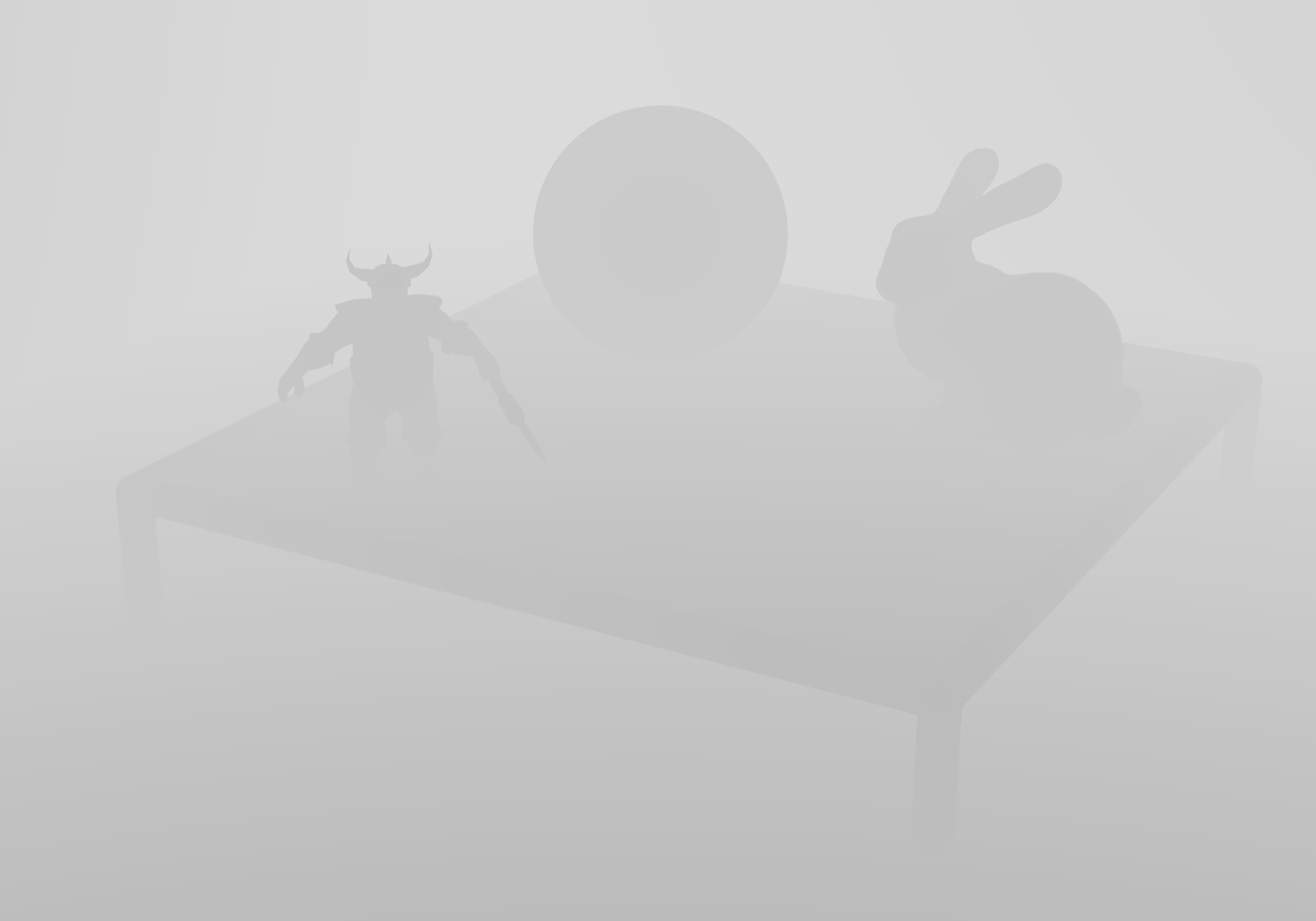
Then t / maxDistance as a smooth grayscale gradient — closer surfaces dark, farther ones bright. Discontinuities mean the wrong ray won the closest-hit comparison. If the gradient across a smooth surface isn’t continuous, the normalization is wrong or the ray direction isn’t actually unit-length.
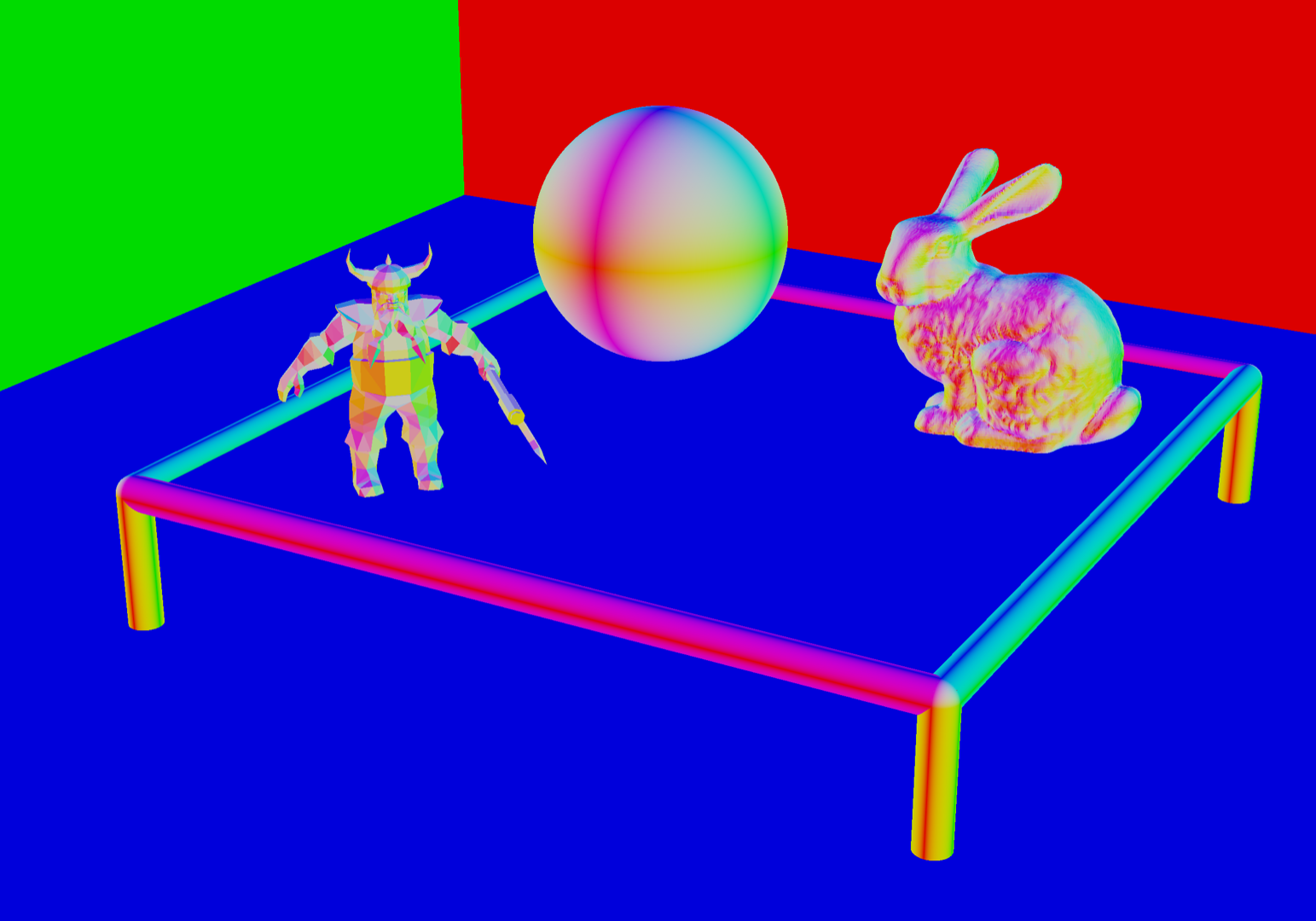
Normals as color are the strictest test. Sphere normals radiate outward — a smooth gradient. Box normals are perpendicular to each face — three flat-colored regions. Triangles show either flat per-face normals or smoothly interpolated ones, depending on whether vertex normals were computed. A normal pointing the wrong way through some boundary shows up as a misaligned color step on the image. The numbers are not wrong in a way a debugger would catch — the orientation is.
Six faces, six colors
Before the BVH is plugged in, each shape’s boundingBox() has to actually contain its shape. An AABB that doesn’t fully contain its primitive will cause rays to skip it entirely; one that’s wildly too large will defeat the acceleration. To verify before trusting the hierarchy, each shape’s intersect() is temporarily swapped for its bounding-box intersection:
// In acceleration.cpp — render the AABB intersect in place of the geometric one
auto result = shape->intersectBoundingBox(ray);
Each boundingBox() is small, but easy to get wrong on the more complex primitives. The cylinder has to enclose both end caps and the full radial extent — box.extend(base ± vec3(radius)) and box.extend(top ± vec3(radius)). The triangle just extends a fresh AABB through its three vertices.
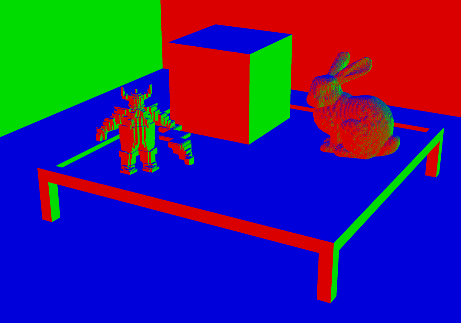
Normals at this level make any error obvious: every face of an AABB is parallel to a coordinate plane, so the normals collapse to exactly six colors. Correctly sized boxes resolve into clean blocks of those six colors, one block per primitive. Anything else — an off-axis tint, a stray gradient, a primitive bleeding through its box — points directly at the constructor that needs revisiting.
Most of the scene, ignored
With four spheres, the renderer is already fast. Add the Stanford Bunny and a Dwarf model — together about a hundred thousand triangles — and a single frame takes 89 seconds. The reason is brute force: for every primary ray, for every pixel, every shape in the scene is asked whether it’s hit. With a 1 megapixel image and 100 000 triangles, that’s 10¹¹ intersection tests per frame. The math doesn’t scale.
A Bounding Volume Hierarchy collapses that toward a logarithm. Shapes are recursively partitioned into a binary tree of AABBs; each interior node’s box bounds all its descendants. A ray descends the tree, but at every node it first tests against the node’s box. If the ray misses the box, the entire subtree is skipped — not one of the primitives below is ever queried. The per-ray cost drops from O(n) to closer to O(log n) in practice, with a small constant overhead from box-test failures along the way.
The renderer pulls in madmann91’s bvh_v2 library rather than rolling its own — its traversal is well-tuned, supports both robust and fast slab tests, and accepts arbitrary leaf intersection through a callback. Plugging it in requires bridging two coordinate worlds: the library uses its own Bvh::BBox<float, 3> for boxes and bvh::v2::Ray for rays, while the rest of the codebase is built on glm::vec3. A pair of thin adapters does the translation. SimpleBox extends the library’s BBox with GLM constructors, and BvhShape wraps a Shape* so that the BVH can hold any primitive uniformly:
struct BvhShape {
    Shape* shape;
    SimpleBox getBoundingBox() const { return shape->boundingBox(); }
    // Called by the traversal when a leaf's AABB is hit
    std::optional<Intersection> intersect(const bvh::v2::Ray<float, 3>& ray) const;
};
The traversal calls back into BvhShape::intersect only after the leaf’s AABB has already been hit, which is what makes the whole thing pay off — the per-shape geometric test runs only when there’s a real chance of hitting it.
Building the tree itself is a separate decision. The library exposes two builders for the same hierarchy, with very different cost models:
SweepSahBuilderuses the Surface Area Heuristic: at each split, it evaluates the cost of placing the partition along every candidate position on every axis, choosing the one that minimizes expected ray traversal cost. It produces high-quality trees but builds single-threaded.MiniTreeBuildertrades some tree quality for parallelism: shapes are bucketed into mini-trees built on independent threads, then stitched into a top-level structure.
Both produce trees that drop the same dense scene from 89 seconds to roughly 130 ms. With the multi-threaded builder, 110.
| Method | Trial 1 | Trial 2 | Trial 3 | Notes |
|---|---|---|---|---|
| Non-BVH | 89423.45 ms | 89623.23 ms | 89784.13 ms | Brute-force, every ray |
| SweepSahBuilder | 130.44ms | 132.91ms | 136.96ms | Single-threaded, SAH |
| MiniTreeBuilder | 111.41ms | 109.23ms | 110.55ms | Threaded build |
A roughly 700× improvement. The math has not changed — every primitive that gets tested is tested with exactly the same intersection routine as before. What changed is how many of them get tested. The BVH lets the renderer ignore most of the scene most of the time, and the gap between mathematically correct and computationally tractable becomes very real.
The trade-off is real at the other end too. For trivial scenes — a handful of primitives — the build cost dominates, the tree is shallower than the constant-overhead penalty, and a flat-list brute force is faster. The BVH only earns its keep once the geometry is dense enough that the savings on traversal outweigh the cost of building the tree. The crossover, in this scene, is somewhere around a few hundred primitives. For path tracing, where the same tree is queried tens of millions of times per frame across primary rays, shadow rays, and bounce continuations, that crossover comes very fast.
What the image doesn’t yet say
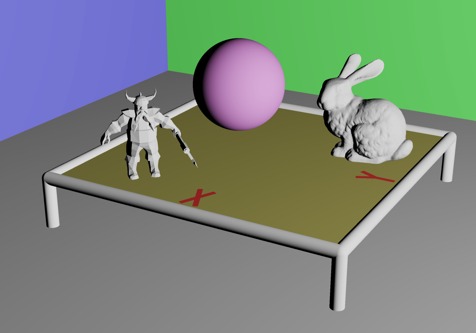
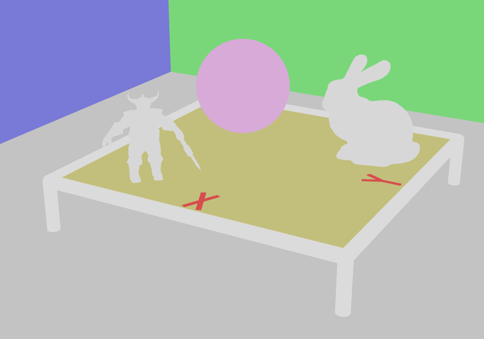
This is what the ray caster produces at the end of chapter one. The pink sphere, the bunny, the dwarf, the table all read as solid objects sitting inside a Cornell-style room — diffuse identity from each material, apparent volume from the surface normal modulating that color’s brightness. Shapes appear in the right place, depth is correct, normals point outward, the BVH delivers its speedup — and at a glance, the composite reads almost like a lit render.
It isn’t. There is no light source in the scene. No ray has illuminated another surface; no energy has moved between two points. The “shading” is just the surface normal scaling each fragment’s diffuse — a viewport-style visualization that tracks form the way a clay model does.
What’s missing is the rendering equation. The next chapter introduces it — direct light first, by shooting a second ray from each hit toward a known source and asking whether it gets there.