The output of the previous chapter is convincing geometry illuminated from nowhere. Each pixel knows what surface it sees and what color that surface was painted, but every visible point is the same brightness as every other point on the same material. Nothing is in shadow, nothing is brighter on the side facing a light, nothing reflects a neighbor. The renderer reports what a ray hit; it has no theory of how that hit was lit.
Path tracing is the move from “what” to “how much.” The framework is the same — primary rays, intersections, BVH traversal — but each pixel becomes the answer to an integral, and the integral is solved by Monte Carlo sampling: many random light paths, each contributing a small unbiased estimate, averaged into the final color.
A pixel covers an area
Before any light bounces, there’s a cheaper correction to make. A pixel covers an area on the image plane, and aliasing — the stair-stepping at every silhouette — is what happens when that area is sampled at exactly one location every frame.
The fix is one line at the top of the per-pixel loop:
float u = (float)(x + myrandom(RNGen)) / width;
float v = (float)(y + myrandom(RNGen)) / height;
Each pass, the primary ray’s footprint within the pixel jitters. After many passes, the pixel’s final color is the average of many slightly different scene samples, and the silhouette resolves into a smooth gradient instead of a hard step. Anti-aliasing isn’t a separate post-process here. It falls out of the same Monte Carlo machinery that’s about to start sampling light.
A path that hopes to find a light
The most direct interpretation of the rendering equation is: trace a ray from the eye into the scene, then keep extending it from each surface in a randomly chosen direction, and hope the path eventually intersects a light. If it does, multiply along the chain of BRDF responses to find that path’s contribution. If it doesn’t, the path contributes zero. This is implicit path tracing: light is found by accident.
The bounce loop reads almost like its description. At each surface, a new direction is sampled from the BRDF, and the ray is extended from a slightly offset origin to avoid self-intersection:
vec3 N = P.normal;
vec3 inDir = SampleBRDF(N);

Ray Q(P.position + EPSILON * P.normal, inDir);
Intersection nextHit = accelStruc->intersect(Q);
The accumulated weight W along the path is updated by the BRDF response divided by the probability of having sampled that direction:
float eval = EvalScattering(N, inDir);
vec3  f    = P.shape->mat->Kd * eval;
float p    = pdfBrdf(N, inDir) * RUSSIAN_ROULETTE_PROB;
W *= (f / p);
If the ray happens to land on a light, the light’s emission is added in, weighted by W, and the path terminates:
if (nextHit.shape->mat->isLight()) {
    C += W * nextHit.shape->mat->Kd;
    break;
}
For a purely diffuse (Lambertian) BRDF, the natural sampling distribution is cosine-weighted on the hemisphere — samples are denser around the normal, where the cosine factor in Lambert’s law is largest:
glm::vec3 SampleBRDF(const glm::vec3& normal) {
    float e1 = sqrt(myrandom(RNGen));    // cos-weighted
    float e2 = myrandom(RNGen) * 2.0f * PI;
    return SampleLobe(normal, e1, e2);
}
The matching PDF is cos(θ) / π, and the BRDF response itself is also cos(θ) / π. The two cancel out on every bounce, leaving the weight update equal to the diffuse color Kd per bounce. The cancellation is correct but not a special case — the same EvalScattering and pdfBrdf calls are kept abstract, so that more complex BRDFs in later chapters can replace them without touching the loop.
Russian roulette, in place of a depth limit
A naive implementation needs a maximum bounce count, or paths run forever. A hard cap is biased: it discards energy that would have come from deeper paths.
Russian roulette terminates probabilistically. At each iteration, a random number decides whether the path continues:
const float RUSSIAN_ROULETTE_PROB = 0.8f;
while (myrandom(RNGen) <= RUSSIAN_ROULETTE_PROB) {
    // ... extend path ...
    float p = pdfBrdf(N, inDir) * RUSSIAN_ROULETTE_PROB;
    W *= (f / p);
}
The path has an 80% chance of continuing and a 20% chance of being cut. To stay unbiased, the accumulated weight is divided by the continuation probability — surviving paths therefore carry a slightly higher weight, statistically compensating for the ones cut early. Across many passes, the estimator still converges to the correct integral.
The trade-off is subtle: longer paths are still possible, just rarer, and a path that survives many bounces gets disproportionately bright weights. That introduces variance, which is fine. Variance only slows convergence; it doesn’t break correctness. What would break correctness is biasing the average, and the division by the continuation probability is what prevents that.
(All convergence images from here on are rendered close to display resolution so the integrator’s per-pixel variance reaches the screen unsmoothed. Higher source resolutions would let the browser average noise across pixels — a free variance-reduction filter that would understate exactly the differences this chapter exists to show.)
Light by accident, image by patience
Implicit path tracing is mathematically clean and visually disastrous. Because the only way to register illumination is to land on a light, most paths contribute nothing, so each pixel’s running average is built from very few non-zero samples. Thousands of passes are needed to average the variance down to a coherent scene.
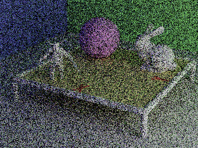
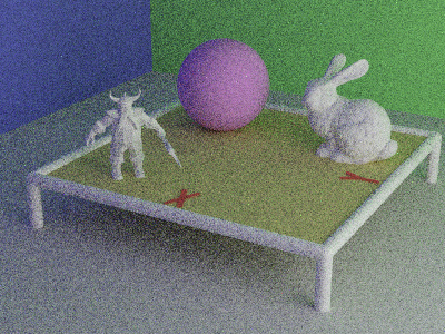
At eight passes per pixel, the image is almost entirely noise. Surfaces are technically sampled with the right distribution, but the signal-to-noise ratio is so poor that the structure of the scene is barely readable.

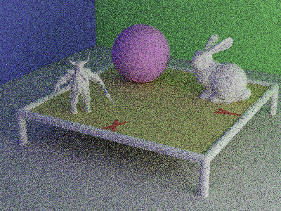
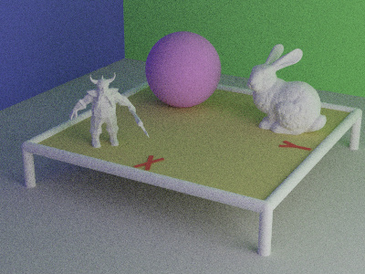
At 256 passes, the noise is reduced but still dominant. The Cornell-box-style room is visible; the sphere, dwarf, and rabbit have shape; but every flat region still shimmers.

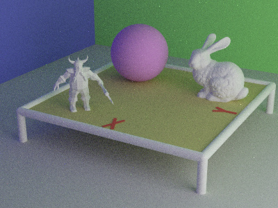
At 4096 passes, implicit tracing is finally producing a clean image. That’s the problem. Four thousand samples per pixel for an image this simple says the strategy is wasteful. The convergence is correct. The compute cost is not.
Pointing the next ray at the light
The fix is to stop relying on luck. At every surface, instead of only extending the path in a random direction and hoping, the renderer additionally casts a deliberate shadow ray straight at a sampled point on a light source. This is explicit path tracing, also known as next-event estimation.
Intersection L = SampleLight();
float p        = PdfLight(L) / GeometryFactor(P, L);
glm::vec3 inDir = normalize(L.position - P.position);

Ray shadowRay(P.position + EPSILON * P.normal, inDir);
Intersection hit = accelStruc->intersect(shadowRay);

if (p > 0 && hit.t < INF && hit.shape->mat->isLight()) {
    float eval = EvalScattering(P.normal, inDir);
    vec3  f    = P.shape->mat->Kd * eval;
    C += W * (f / p) * hit.shape->mat->Kd;
}
SampleLight picks a random point uniformly on the light’s surface — a sphere, in this scene. The mapping that gets you there isn’t quite the obvious one. Sampling spherical coordinates (θ, φ) uniformly clusters points at the poles; the honest uniform-on-sphere distribution samples z linearly and recovers the radial coordinates from it:
float z = 2.0f * e1 - 1.0f;            // uniform z ∈ [-1, 1]
float r = sqrt(1.0f - z * z);
float a = 2.0f * PI * e2;
vec3 N = vec3(r * cos(a), r * sin(a), z);
vec3 P = center + radius * N;
The same trick recurs every time the renderer needs an unbiased sample on a sphere. GeometryFactor then corrects for the change of variables from area-on-the-light to direction-on-the-hemisphere — geometrically, the cosine on the light’s surface times the cosine on the receiving surface, divided by the squared distance between them. The shadow ray’s job is one binary question: does the ray reach the light unobstructed? If yes, the light’s contribution is added to the path’s accumulated color, weighted by the BRDF response and the geometry factor. If no, the path simply doesn’t get that direct connection — but it still continues with the implicit bounce, so no energy is lost.
Because the explicit and implicit strategies can both contribute light from the same source on the same bounce, both contributions are weighted by 0.5f to avoid double-counting. (A more principled weighting comes in the next chapter; for now the equal split is correct on the diffuse-only scene.)
The same image, far fewer rolls
Explicit shadow rays don’t change what the renderer is solving; both methods converge to the same image. They change how fast. Every unoccluded surface receives a direct light contribution at every bounce, so the image starts out bright and consistent rather than sparse and confetti-noisy.
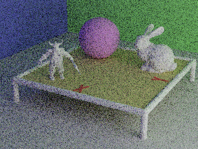
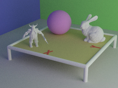
At eight passes, explicit path tracing has already drawn most of the scene. The shapes, the soft shadows, the colored bounce off the walls — all visible. There’s still noise, but the structure of the image is there.
At 256 passes, the explicit render is approaching what implicit tracing took 1024 passes to produce. Soft shadow boundaries beneath the rabbit and the dwarf are clean. The colored indirect lighting from the green and blue walls reads correctly across the diffuse surfaces.
Side by side at identical pass counts, the gap shows up immediately:


In rough terms, explicit at 16 passes is comparable in quality to implicit at 32, and that ratio widens as the scene gets harder. The two methods agree at the limit; past about 512 passes the renders become visually indistinguishable, which is the empirical statement of the fact that both are unbiased estimators of the same integral. Explicit just gets there with an order of magnitude less work.
Every surface here is still diffuse
The renderer can now compute correct global illumination, accelerate it with explicit lighting, and produce visually clean images at modest pass counts. But every surface in this scene still uses the same Lambertian BRDF — flat, perfectly diffuse, with a Kd color and nothing else. There is no glossy highlight, no metallic shine, no Fresnel falloff at grazing angles. A polished marble sphere and a sheet of construction paper would render identically.
That assumption is the next constraint to break. Real surfaces aren’t flat at the wavelength of light; they’re rough at a scale this scene hasn’t needed yet, and their BRDF is the statistical aggregate of the microfacets that compose them. The next chapter is what happens when EvalScattering stops being one line.