The renderer at the end of the previous chapter describes opaque materials well: diffuse, glossy, metallic, and everything between. Every ray that strikes a surface either reflects back into the world or is absorbed into the BRDF’s diffuse sum. None of them continue through the surface. Glass, water, gemstones, tinted plastics — the entire category of dielectric materials that bend light rather than block it — cannot be expressed in the current framework.
This chapter adds a third channel to the BRDF: transmission. A ray hitting a transmissive surface can pass through it according to Snell’s law, lose energy to absorption proportional to the distance travelled inside the medium (Beer’s law), and emerge on the other side bent and tinted. Three places in the renderer change — the sampler, the PDF, and the evaluator — and they all share the same new piece of bookkeeping: the index of refraction, and which side of the surface the ray is on.
Snell at every microfacet
Two new fields appear on Material:
vec3  Kt;   // Color of light remaining after one unit of travel through the medium
float ior;  // Index of refraction (1.0 = air, ~1.5 = glass)
Snell’s law relates the angles on either side of a surface boundary by the ratio of the indices. To stay consistent across all three channels (sample, eval, PDF) the renderer needs to know, at every hit, which way the ray is crossing the boundary — entering or leaving — because the ratio η = ηᵢ / ηₒ flips depending on which side is which. A small helper centralizes that:
std::pair<float, float> computeEta(vec3 outDir, vec3 N, Material* mat) {
    float outDotN = dot(outDir, N);
    if (outDotN > 0.0f) return { 1.0f, mat->ior };  // leaving:  air -> material
    else                return { mat->ior, 1.0f };  // entering: material -> air
}
By convention the outgoing direction outDir (ωₒ) points back toward the camera. If it’s on the same side as the surface normal, the path is exiting the material; if on the opposite side, it’s about to enter. The same computeEta is called from the sampler, the PDF, and the evaluator. All three need to agree on which direction the ray is heading.
The sampler now picks between three lobes — diffuse, specular reflection, transmission — proportional to the magnitudes of Kd, Ks, and Kt. The diffuse and reflection branches are unchanged from the previous chapter. The transmission branch samples a microfacet normal m from the same Phong NDF, then refracts the outgoing direction through that microfacet using Snell’s formula:
auto eta = computeEta(outDir, N, mat);
float ior = eta.first / eta.second;
float outDotM = dot(outDir, m);
float r = 1.0f - (ior * ior) * (1.0f - (outDotM * outDotM));

if (r >= 0.0f) {
    int sign = dot(outDir, N) >= 0.0f ? 1 : -1;
    return (ior * outDotM - sign * sqrt(r)) * m - ior * outDir;
}
The radicand r = 1 − η²(1 − (ωₒ·m)²) is the standard Snell discriminant. When it’s non-negative, a real refracted direction exists and the formula returns it. When it’s negative, there’s no valid refraction angle: the ray has hit the boundary at an angle steeper than the critical angle for this index ratio.
When the ray cannot leave
Total internal reflection (TIR) is what happens when light hits the inside of a denser medium at a steep enough angle that no refracted direction can carry it out. Inside a glass sphere, rays grazing the inner surface can’t escape; they bounce internally until they happen to hit the surface at an angle below the critical threshold. This is what produces caustics, the bright concentration at the bottom of a glass of water, and the prismatic effect inside a faceted gemstone.
The sampler handles TIR by falling back to specular reflection, the only physically valid option:
if (r < 0.0f) {
    // Total internal reflection: no real refraction direction exists
    return 2.0f * dot(outDir, m) * m - outDir;
}
The evaluator and the PDF both have to recognize the same case and use the same fallback. If the sampler refracts and the evaluator computes a transmission term, the estimator stays consistent. If the sampler reflects (TIR) and the evaluator computes a reflection term, the same. What breaks the estimator is when the three disagree about whether the radicand was negative. That’s why all three call computeEta and run the same 1 − η²(...) test.
Color that thickens with distance
The Kt field is the color of light remaining after travelling one unit of distance through the medium, not a flat tint applied at the surface. For a path length t inside the material, the attenuation is
A(t) = exp(t · log(Kt))derived from Beer’s law A(t) = e^{-ct} with c = -log(Kt). A red-tinted glass (Kt = (0.9, 0.1, 0.1)) lets through almost all of the red but absorbs most of the green and blue per unit length, so a thicker cross-section of the same material becomes more saturated and darker. A neutral glass (Kt ≈ (0.9, 0.9, 0.9)) loses a small amount of energy uniformly across all channels.
The path length t the renderer needs is exactly the parametric distance between consecutive intersections: the same t this entire series has been built around. It’s already on the Intersection struct from chapter 1. Beer’s attenuation appears in EvalScattering only when the ray is inside the medium (i.e. outDir · N < 0, meaning it just hit an inner surface):
vec3 atten = vec3(1.0f);
if (outDotN < 0.0f && t > 0.0f) {
    atten = glm::exp(t * glm::log(mat->Kt));
}
The attenuation factor multiplies the transmission term, both in the refraction case and in the TIR case. Energy is reduced no matter what; it’s just a question of which direction the ray takes after losing it.
Two half-vectors, two equations
The microfacet specular reflection from the previous chapter uses one half-vector: m = normalize(L + V). Microfacet transmission needs a different one. The microfacet that turns V into a refracted L is not the bisector but the vector that satisfies Snell’s law for a virtual mirror reflection at the boundary, which works out to:
tm = -normalize(η_o · L + η_i · V)This second half-vector enters the evaluator’s transmission branch:
vec3 tm = -normalize(no * L + ni * V);
float LdotM = dot(L, tm);
float VdotM = dot(V, tm);

float D = DistributionPhong(N, tm, alpha);
float G = GeometrySmith(N, L, V, tm, alpha);
vec3  F = vec3(1.0f) - FresnelSchlick(L, tm, mat);   // (1 - F): the part NOT reflected

float denom = (no * LdotM) + (ni * VdotM);
denom *= denom * abs(outDotN);

vec3 num = atten * D * G * F * abs(LdotM) * abs(VdotM) * (no * no);
transmission = (denom > 1e-6f) ? (num / denom) : vec3(0);
The PDF computes the same Jacobian on the same tm, which is how the f / p ratio stays unbiased across refractive bounces:
float pDenom = (no * LdotM) + (ni * VdotM);
pDenom *= pDenom;
Pt = (D * dot(tm, N) * (no * no) * abs(LdotM)) / pDenom;
The shared no² / (no·LdotM + ni·VdotM)² factor is the change-of-variables Jacobian from microfacet-normal space to outgoing-direction space. If eval and PDF compute it differently (even slightly), every refractive bounce becomes biased even though both functions look correct in isolation.
(1 − F) matters here: Fresnel reports the fraction reflected, so transmission gets the complement, the energy that crossed the boundary. When the radicand goes negative, eval and PDF both fall back to the reflection formula, mirroring the sampler’s TIR fallback. The three places have to agree on the same case, or the estimator drifts.
The epsilon offset picks a side
Chapter 1’s epsilon trick — offsetting the new ray’s origin by a small amount along the normal — works for reflection because reflected rays leave the surface on the side the normal points to. Transmitted rays go the other way. Offsetting them along +N puts the new origin on the wrong side of the boundary, the next intersection query finds the same surface again, and the path either self-terminates or accumulates a string of false hits inside its own surface. A glass sphere rendered this way loses its transmission entirely.
The fix is to let the offset direction track which side the new ray is heading toward:
bool isTransmission = dot(inDir, N) < 0.0f;
Ray Q(P.position + (isTransmission ? -1.0f : 1.0f) * EPSILON * N, inDir);
If the sampled inDir points into the surface (inDir · N < 0), the offset flips to −N and the new origin sits on the inside of the boundary, ready to traverse the medium. If it points out — reflection, diffuse bounce, TIR fallback — the offset stays +N as before. The single sign flip is the difference between a glass sphere that refracts and one that doesn’t render at all.
A sharper heuristic for sharper lobes
The balance heuristic from chapter 3 quiets fireflies on glossy surfaces by weighting each strategy in proportion to its PDF. On transmissive surfaces — where the BTDF concentrates rays into an even narrower lobe than the BRDF’s specular peak — the balance heuristic isn’t aggressive enough. The fix is the power heuristic, which squares the PDFs before normalizing:
// Explicit light connection
float weight = (p_light * p_light) / (p_light * p_light + p_brdf * p_brdf);

// Implicit BRDF-sampled connection
float weight = (p_brdf * p_brdf) / (p_brdf * p_brdf + p_light * p_light);
Squaring exaggerates differences. When one PDF dominates the other, the dominant strategy gets a weight close to 1 and the other close to 0. On strongly directional lobes — specular reflection, transmission — that’s the right behavior: only one strategy is ever well-suited to sampling them, and equal weights would just inject noise from the wrong one. On diffuse surfaces, both PDFs are comparable, so squaring them changes the balance only slightly, and the result still converges to the same image.
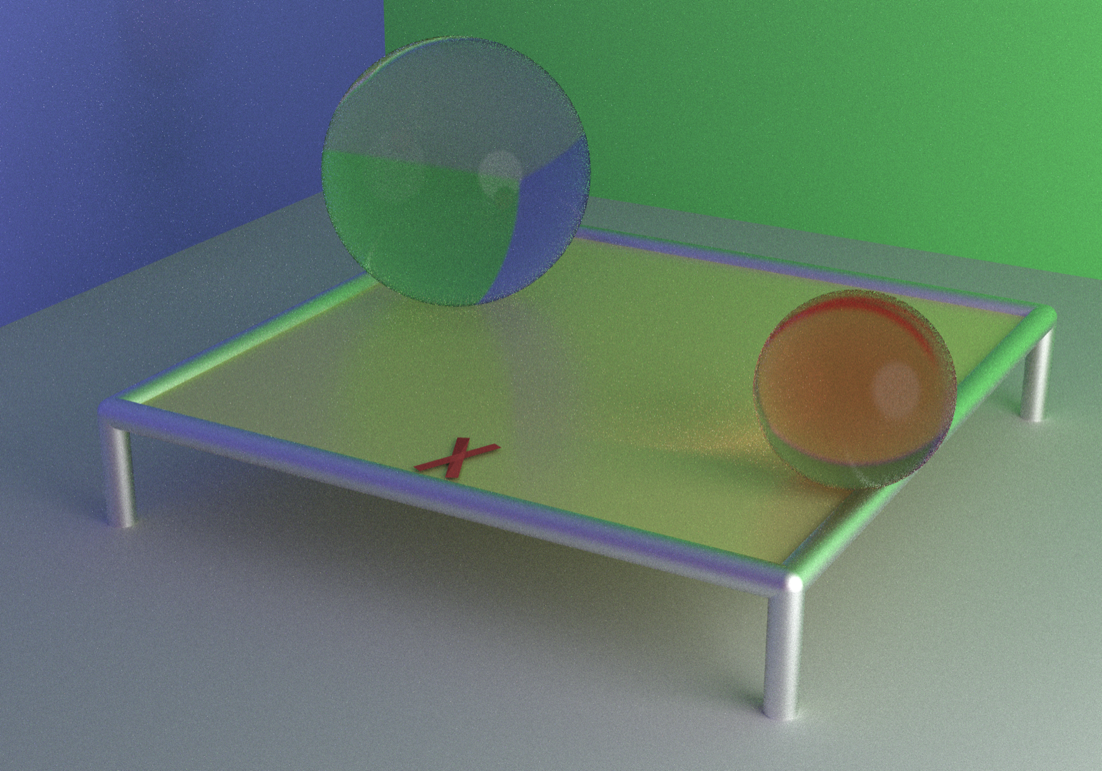
A 128-pass render under flat equal-weight MIS: fireflies saturate the transmissive geometry, because the BRDF sampler keeps drawing rays at low probability that happen to graze the bright light through the glass.
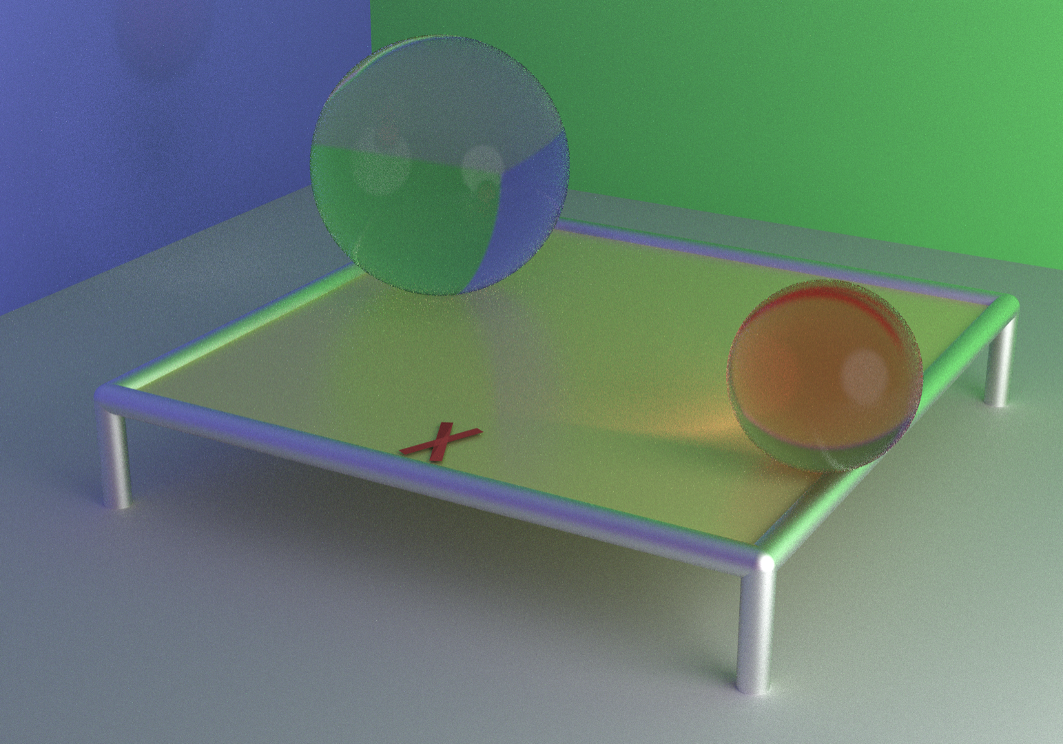
The same scene at the same pass count with the power heuristic. The fireflies collapse into clean transmitted highlights, the caustic patterns inside the spheres resolve, and the image looks closer to what the math has been computing all along.
Glass, on three test scenes
With sampler, evaluator, PDF, and MIS aligned on the new lobe, the path tracer can render glass.
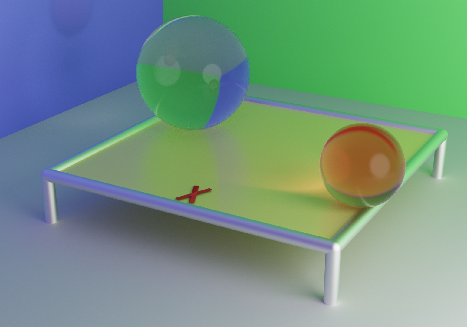
Scene 1: two glass spheres on the reflective table from chapter 3. The larger sphere uses near-neutral glass (Kt ≈ (0.9, 0.9, 0.9), ior = 1.25), the smaller uses red-tinted glass (Kt = (0.9, 0.1, 0.1), ior = 1.25) that absorbs almost all of the green and blue. The refracted image of the scene seen through the red sphere is correspondingly red, while the neutral sphere produces an almost colorless refraction.
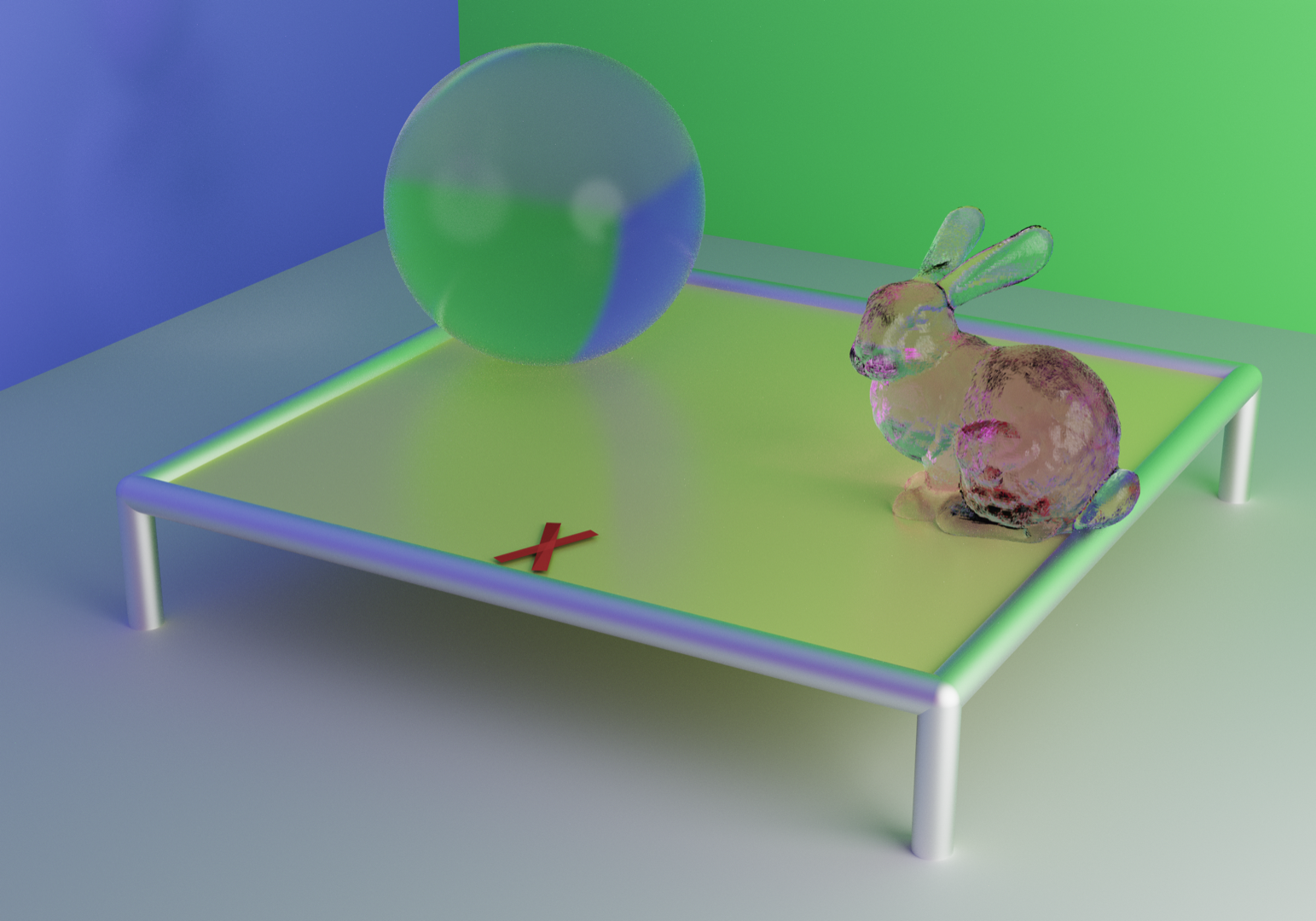
Scene 2: a glass-tinted Stanford bunny. The bunny uses pink glass (Kt = (0.9, 0.1, 0.9), ior = 1.5), which absorbs green more than red or blue. The non-convex geometry exercises every part of the transmission system: rays must refract on entry, possibly TIR on tight curves of the ears, accumulate Beer attenuation across the chord they travel through the body, and refract again on exit. Thicker cross-sections (the torso, the haunches) appear deeply tinted; thin regions (the ears) transmit almost cleanly. The neutral glass sphere alongside acts as a control.
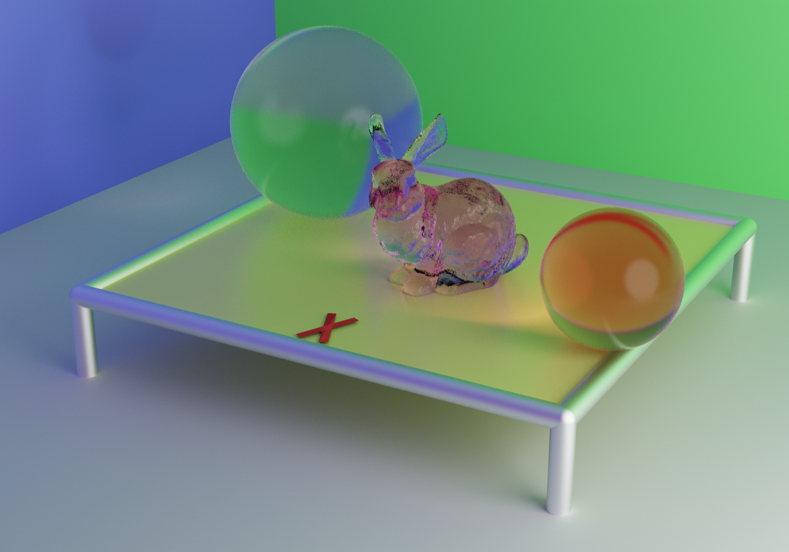
Scene 3: all three transmissive objects together — the red sphere, the neutral sphere, and the pink bunny. Rays now traverse multiple media in sequence, accumulating refraction at each boundary and Beer attenuation over each medium’s chord. Through the bunny’s right ear, the larger neutral sphere is visible behind it, and the sphere’s own refraction distorts the colored side walls into a curved compressed image, all visible through the bunny’s silhouette.
What the room around it still doesn’t do
The renderer can now describe surfaces that absorb, reflect, and transmit light, with materials that range from chalk to mirror to glass. What it can’t yet do is light a real room. Every scene in this chapter is illuminated by a single hand-placed sphere light hovering above a small set of objects, surrounded by colored walls. The lights are simple, the geometry counts are in the thousands, and the only environment is whatever those walls happen to bounce.
Reaching the kind of scene the eye expects from a path tracer — a city street at night, a courtyard under afternoon sun, an interior lit by a sky and a hundred small lamps — is an infrastructure problem more than a math problem. The next chapter is about that infrastructure: how to load millions of triangles without choking, how to treat a sky as a light source, how to treat all of the scene’s emissive geometry as a single distributed light, and how to iterate on something that takes minutes to render per frame.